Since 2018, all operational forecast systems at ECMWF have modelled the evolution of the ocean and sea ice using a dynamical model, based on NEMO3.4.1 and a single-category ice model LIM2 (Keeley & Mogensen, 2018). For the last five years, we have been working to develop an updated ocean and sea-ice model and data assimilation system for use in all of ECMWF’s physical modelling systems. The next upgrade of the ocean component of the model will be an updated ocean model based on the code base NEMO4.0.6 of the NEMO community model (https://www.nemo-ocean.eu/). This features, among other things, a new spatial grid, new options for the formulation of the surface fluxes, and a new community multi-category sea-ice model SI3 (Sea Ice modelling Integrated Initiative), which builds upon the models previously used within NEMO: LIM3, CICE and GELATO.
In addition to the scientific changes, several technical changes have been introduced, leading to significantly better computational performance in terms of scalability, which reduces the time to solution. The new version of NEMO has been integrated in the ECMWF infrastructure, and it has been further developed and configured. Thus, the upgrade of the ocean modelling component will mirror the fact that ECMWF’s Integrated Forecasting System (IFS) makes use of a single-precision version of the model for forecasts while retaining double precision for the analysis. The ocean output will become available in ECMWF’s Meteorological Archival and Retrieval System (MARS) in GRIB2 via the MultIO server. There will be no change in resolution; the challenge has been to improve the realism and variability of the ocean surface and to ensure consistency in the surface flux formulation between coupled and uncoupled experiments. The first operational application of NEMO4-SI3 will be the production of the new generation of ocean reanalysis (ORAS6, see article by Zuo et al. in this Newsletter), and its coupling with ERA6. It will also be used by the upcoming seasonal forecasting system SEAS6. The plan is for NEMO4-SI3 to be the ocean component of all ECMWF forecasting and monitoring systems from IFS Cycle 50r1, which is to be introduced in 2025. The details of the ocean data assimilation upgrades and the corresponding ocean reanalysis are discussed in more detail in the article on ORAS6 in this Newsletter. This article focuses on the features of the updated elements of the model in terms of ocean forecasts and impacts on the atmosphere. For the rest of this article, we refer to the new model version as NEMO4 and the model it is replacing as NEMO3.4.
Main developments from NEMO3.4 to NEMO4
The NEMO community model has undergone much change since our last operational version was implemented. The code has many differences both technically and scientifically, including the replacement of LIM2 with SI3. When implementing the NEMO4 ocean model, we have tailored it for our use within our operational systems, alongside the reimplementation of changes we previously made in house to NEMO3.4 to improve computational efficiency. These changes are made based on the forecast time horizons we are interested in, robustness and computational efficiency of the code for operational implementation, and the ability to initialise the forecasts. This required many hundreds of model simulations to be run, assessing the impact of the choices that can be made to optimise the model setup. There are also a number of new options in NEMO4 that have been provisionally tested during the development phase. They include the representation of icebergs and new sea-ice rheologies, and they can be activated at a later date should they be found to improve performance. This article reviews the key features of NEMO4 and summarises the key performance metrics for the new system. The main change in physical representation in the upgrade from NEMO3.4 is the formulation of the way the ocean surface is represented. We now use a variable volume formulation for the upper surface layers of the ocean. The upper ocean turbulent mixing is modified when sea ice is present, in which case the impact of waves on the mixing is attenuated.
Collaboration with Member States
Implementation of the new model drew on ECMWF Member State expertise with ocean sea ice model development work. The NEMO team at LOCEAN in France provided support, especially with the new sea ice model code as we tested it for operational use. During much of the development phase, we have worked alongside the UK Met Office Joint Marine Modelling Programme, which draws on oceanographic modelling expertise across the Met Office and UK research community. Our NEMO4 model grids and bathymetry are based on the UK Met Office configuration of its Global Ocean 8. The model grid and bathymetry use the extended ORCA (eORCA) grid (Madec & Imbard, 1996); the ocean model boundary is further south and now extends beyond 78°S to 86°S. The extended grid is required for any future development work to model the ocean interaction under Antarctic ice shelves, although this is not currently considered. The resolution remains the same as in the current operational model, with 75 levels in the vertical and a tri-polar grid with a nominal 0.25-degree horizontal resolution.
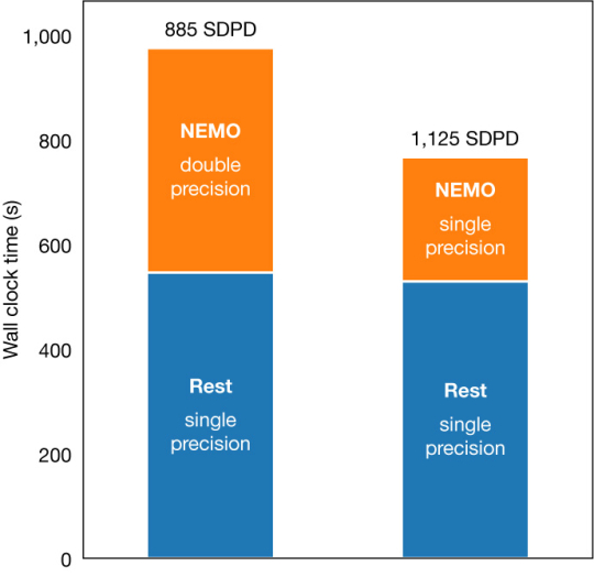
Building on earlier work by the Barcelona Supercomputing Center, we have also added the capability to run NEMO4 using single-precision arithmetic (see Rodwell et al., 2021). We carried out extensive testing to make sure that our version of NEMO4 can run stably with single precision, and that there is no impact on forecast scores. Nevertheless, as with the atmospheric component of the IFS, we will keep using double precision as a default for the ocean analysis. We find that the single-precision implementation can accelerate NEMO by up to 1.8 times, compared with the double-precision version. However, this depends strongly on the context in which NEMO is running. In cases where NEMO is running at the limits of its scalability (for example, when using many hundreds of nodes for eORCA12 simulations), the gains from using single precision diminish dramatically. For the seasonal and extended-range forecasting systems, where the ocean cost is a large part of the total run time, the effect is very important, as illustrated in Figure 1.

Atmospheric forcing of the ocean
When developing the model and generating the ocean analysis, we run the model with atmospheric forcing. This is referred to as bulk forcing of the ocean and represents the momentum, heat, and moisture exchange over the ocean. The exchange of fluxes between the atmosphere and ocean is based on roughness length scales for these three processes in the IFS. The quality, frequency and available variables of a driving dataset can influence the performance of the ocean–sea-ice model. Since the last ocean model was implemented, improvements have been made in the forcing data from the atmosphere, which are now from ECMWF’s ERA5 reanalysis rather than ERA-Interim. Not only is the quality of the driving data improved on that of the previously used ERA-Interim reanalysis, but the higher frequency (hourly) forcing has contributed to a better representation of the diurnal cycle. Results of this can be seen in Figure 2 of the article on ORAS6 by Zuo et al. in this Newsletter. New bulk formulation options that have been added within NEMO4 allow increased consistency between the surface fluxes used in uncoupled ocean mode (which is used for the production of ocean reanalysis) and coupled mode (which is used for the coupled forecasts). Given that the wave model is an integral part of our forecasting system and mediates the surface exchange between the atmosphere and ocean, we run the NEMO4 system with the surface wave impacts. The aim is to improve the upper ocean representation and aid the development of the ocean model for coupled implementation within our forecasting systems. Wave data are also available from ERA5. The use of wave forcings was first introduced in our version of NEMO3.4 (Breivik et al., 2013), and many of these wave forcings are now available options in NEMO4. To be consistent with our earlier version of NEMO, we have re-introduced the impact of wave breaking on the turbulent kinetic energy (TKE) surface flux in the parametrization of the upper ocean mixing. Where data that is required is not available from ERA5, it has been recomputed from existing available data.
For momentum under windy conditions, the IFS uses a sea-state-dependent Charnock relation. We modified NEMO4 from using a constant Charnock coefficient to a varying Charnock field that is consistent with the other wave forcing fields. The surface fluxes in NEMO4 are adjusted iteratively to account for the presence of surface currents. Naively, when using atmospheric forcing that has not used information on surface currents, such as ERA5, one would assume that the surface fluxes should be computed based on 10 m winds relative to the surface currents. However, we have shown that, if the atmospheric model had used surface current information, the whole near-surface wind profile would be modified in response to the modified surface condition. On average, in order to yield similar surface stress values using the data from the system without surface currents, one should compute the atmospheric forcing with about half the current effect. Therefore, we opted to only apply half of the surface current effect in the relative wind correction in NEMO4.
ERA5 and operational wave data are not available when sea-ice cover is above 30% due to the lack of a physically consistent representation of wave–sea-ice interactions. Therefore, when sea ice is present in the forcing field, the wave forcing data are determined using simple empirical formulations based on 10 m wind and sea-ice cover or simply using a constant default value.
New sea-ice model – SI3 (sea ice cubed)
Perhaps the largest change in the model setup is the way sea ice is represented. LIM2 is no longer available; NEMO4 contains the new community SI3 model. Operationally LIM2 represents sea ice with a single category and two thermodynamic layers, with a single layer of snow on top. Sea ice has a fixed salt concentration and no possibility of melt pond formation.
The sea-ice rheology of LIM2 is based on continuum dynamics and uses a viscous plastic rheology. For SI3 we make use of a computationally more efficient formulation of this rheology, the elastic-viscous-plastic formulation (EVP).
SI3 brings many new features to the way the thermodynamics of sea ice is modelled at ECMWF that improve the representation of the seasonal evolution of the ice:
- multi-category ice (see Box A for more details)
- spatially and temporally varying sea-ice salinity
- melt ponds
- new prognostic variables to describe the thermodynamic sea-ice properties.
A
Multi-category ice

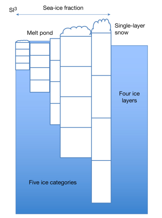
Schematic of the five-category, 4 + 1 ice and snow layer model.
The model represents the subgrid-scale heterogeneity in ice thickness through a multi-category formulation. Ice thickness is therefore another dimension in the prognostic variables, and the thickness distribution is discretised into five categories with fixed thickness ranges. Each category has an associated concentration, discretised into a number of evenly spaced layers, and the thermodynamics of the model is solved for each category. As ice forms or melts, there is a redistribution in the fraction of each thickness category that is present at each model point. It should be noted that the dynamics of the model is solved for each grid box of the model and not for individual categories, and it represents the ridging and rafting of ice when under compression.
The model has been developed with five thickness categories, each with four thermodynamic layers and a single snow layer on top. This configuration is a compromise to represent the complexity of the ice without being too computationally expensive. This change in model formulation required a change in the way sea-ice increments are applied in the data assimilation system (see the article by Zuo et al. in this Newsletter).
The other improvement in the new model that is important for the surface exchange over sea ice is the representation of various surface processes and properties. For example, a level pond scheme is activated, and each category has its own pond fraction and volume. The pond can have a frozen lid, which also affects the surface albedo of the pond. The albedo scheme has been slightly reformulated from that used in LIM2, and the effect of melt ponds is also included. Snow on sea ice is also considered in more detail: as snow falls onto the ice, some fraction gets blown into the ocean, and snow is also lost to the ocean as the ice ridges and rafts. The representation of snow loading has become more critical for the surface exchange as we wish to make use of the snow depth from the ocean analysis to initialise the snow on sea ice within the IFS surface analysis. Representing snow on sea ice helps to reduce warm temperature biases in winter that have been reported both operationally and for ERA5 (see Arduini et al., 2022, for more discussion).
Comparing standalone NEMO4 with NEMO3.4
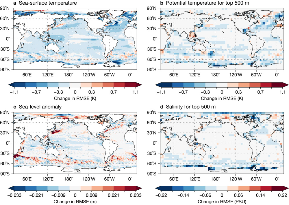
To assess the performance of the ocean model, key model fields are compared to observational datasets. In preparation for providing a model basis for the analysis system for ORAS6, we compared free-running experiments of the uncoupled ocean model, both the operational NEMO3.4 model and the NEMO4 model. Early development work was done using a 1° ocean model and then further refined and tested at 0.25°. We present results here for the latter. Each model is started from a climatological state and run from 1979 for 40 years with hourly ERA5 forcing without data assimilation. The focus of the development work was to provide a model setup that was as good as NEMO3.4, or better, on which to build the assimilation system. We present results with the final setup that was provided for the data assimilation system. To avoid any spin-up from the climatological state in the upper ocean and sea ice, our analysis focused on the second half of the integration (the last 20 years) and is compared to upper ocean observations. Figure 2 shows the differences in root-mean-square error (RMSE) between NEMO4 and NEMO3.4 simulations for sea-surface temperature (SST – verified against ESA-CCI SST v2 analyses), upper ocean 500-metre temperature and salinity (verified against in-situ observations), and sea-level anomaly (verified against altimeter data). The free-running NEMO4 shows errors are broadly reduced compared to NEMO3.4 for all the observed quantities, except for an increase in sea-level anomaly RMSE in eddy-rich regions. Improvements can be seen in SST in areas with known errors in the Southern Ocean and the North Atlantic Current region.

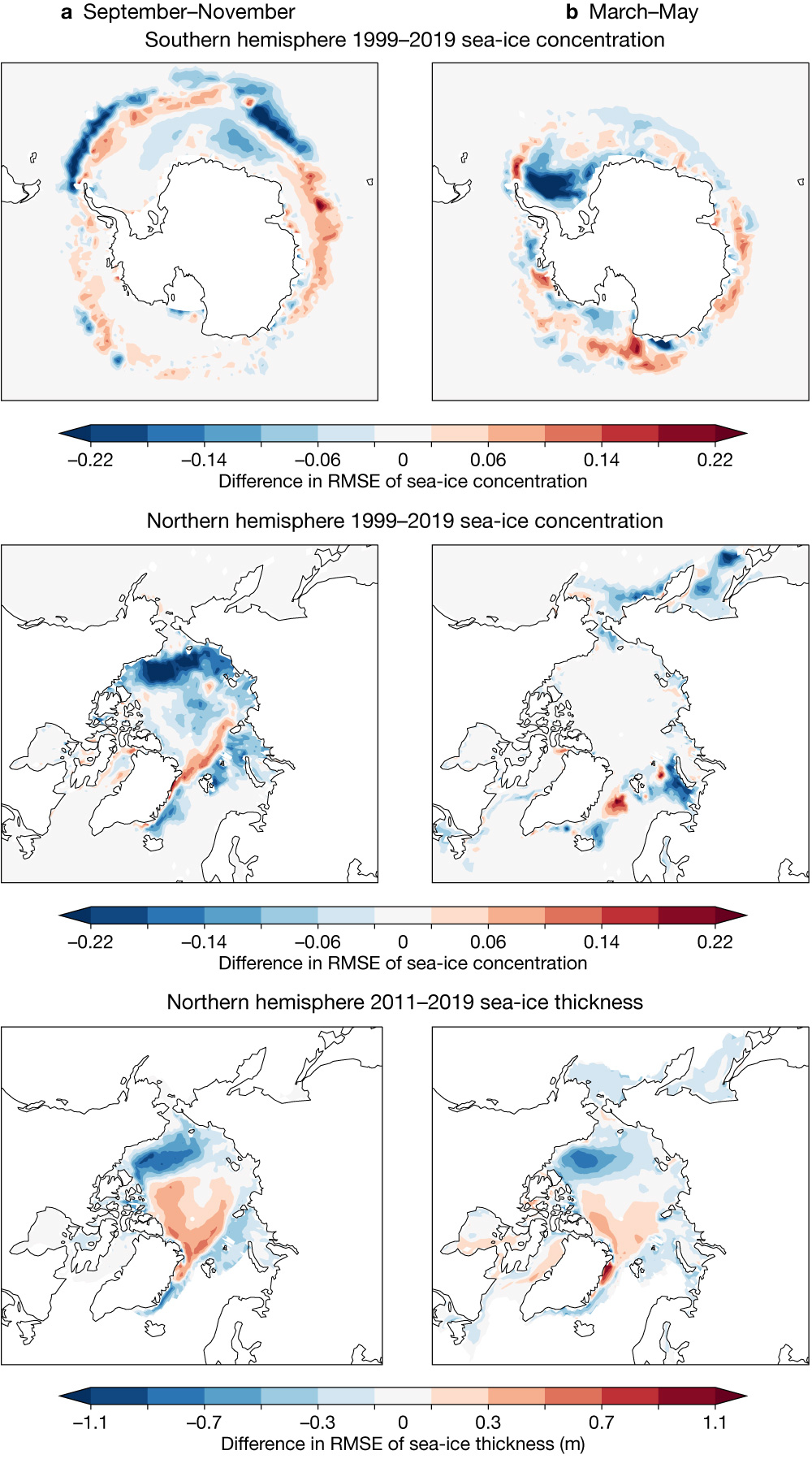
The multi-category sea-ice model freezes and melts sea ice more rapidly than a single category model. We would, therefore, expect the new model to help reduce errors in the marginal ice zone (MIZ). Figure 3 shows the change in RMSE for NEMO4 compared to NEMO3.4 for autumn and spring, when the marginal ice zone is at its minimum and maximum, respectively, for concentration and thickness in the northern hemisphere, where satellite data products exist. In the northern hemisphere, there is a broad reduction in errors in sea-ice concentration, although there are some increased errors in the transition between the MIZ and the perennial ice in the region that extends from northeast Greenland towards northern Russia. In the southern hemisphere, the results are more mixed for the maximum ice extent, with increased errors in the Davis Sea. Large reductions in error are seen in autumn in the Weddell Sea, which is an area sensitive to the snow loading on the ice. The multicategory model is also found to have thinner ice on average in the Arctic (not shown), compared to satellite derived sea-ice thickness products from CryoSAT2 and SMOS. The model removed the positive thickness bias in the Beaufort gyre but has increased the negative thickness bias to the north of Greenland. This leads to increased RMSE in the central Arctic in the sea‑ice thickness field, shown at the bottom of Figure 3.

Easier access to ocean data
The implementation of NEMO4 brings with it a change in the way we archive data from the ocean. In the past, the data was output in NetCDF format and could not be stored in the MARS archive. The technical work to deliver ocean output that is more accessible is described in more detail by Sarmany et al. (2024). It will allow users to access the data from across Earth system model components in the same way.
Impact on coupled system
One of the biggest improvements with the change of sea-ice model and the representation of surface processes is that we can now consider coupling more of the thermodynamic components of the ice. Early testing showed that the marginal ice zone (MIZ) being better represented by the multi-category ice was detrimental to coupled forecasts when using the fractional ice-cover coupling that is used operationally. The operational system assumes that the ice is 1.5 m thick and has no snow on top. These assumptions lead to a warm bias in the polar regions, where the snow insulation effects are not correctly represented, and a cold bias when the thinner ice in the marginal ice zone would allow heat fluxes from the ocean to the atmosphere. Without being able to represent the melt ponds, the summer albedo was not low enough in LIM2, so we made use of a uniform climatological albedo over sea-ice surfaces in the IFS. With this simplification, we found that the modelled sea-ice response is slower than observed. This was particularly true in summer, when there are strong albedo feedbacks. The new elements of SI3 mean that we can make improvements to the sea‑ice/atmosphere interface and reduce model biases that are seen in the reanalysis and forecast systems. We can now implement closer coupling between the sea-ice surface and the atmosphere, coupling the albedo, snow depth and temperatures. Ongoing testing is finalising the coupling framework for the use of NEMO4 within our forecast systems.
Conclusion
Considerable work was done to make sure that the NEMO4 code base that will be implemented in operations is robust and tuned, to provide a system with a baseline requirement to perform as well as its predecessor NEMO3.4. Alongside the scientific development, there have been technical developments to enable the output from the model to be archived in MARS using GRIB2.
NEMO4 is now being used in production of the next ocean reanalysis ORAS6 and will be used for the operational ocean analysis OCEAN6. More details about the specific development work for the assimilation system have been documented by Zuo et al. in this Newsletter. The model will also form the ocean component for all the coupled systems from IFS Cycle 49r2 onwards. The first time this will be implemented in the operational forecast will be in IFS Cycle 50r1.
Further reading
Arduini, G., S. Keeley, J. J. Day, I. Sandu, L. Zampieri & G. Balsamo, 2022: On the Importance of Representing Snow Over Sea‐Ice for Simulating the Arctic Boundary Layer, Journal of Advances in Modeling Earth Systems, 14/7. https://doi.org/10.1029/2021MS002777
Breivik, Ø., M. Alonso-Balmaseda, J.-R. Bidlot, P.A.E.M. Janssen, S. Keeley & K. Mogensen, 2013: Closer together: coupling the wave and ocean models. ECMWF Newsletter No.135, 6–7. https://doi.org/10.21957/ha77zhpn
Keeley, S. & K. Mogensen, 2018: Dynamic sea ice in the IFS, ECMWF Newsletter No. 156, 23–29. https://doi.org/10.21957/4ska25furb
Storkey, D., A.T. Blaker, P. Mathiot, A. Megann, Y. Aksenov, E.W. Blockley et al., 2018: UK Global Ocean GO6 and GO7: a traceable hierarchy of model resolutions, Geosci. Model Dev., 11, 3187–3213. https://doi.org/10.5194/gmd-11-3187-2018
Rodwell, M., M. Diamantakis, P. Düben, M. Janoušek, S. Lang, I. Polichtchouk et al., 2021: IFS upgrade provides more skilful ensemble forecasts. ECMWF Newsletter No. 168, 18–23. https://doi.org/10.21957/m830hnz27r
Sármány, D., K. Mogensen, M. Valentini, R. Aguridan, P. Geier, J. Hawkes et al., 2024: New software libraries for ORAS6 ocean reanalysis, ECMWF Newsletter No. 178, 13-15. https://doi.org/10.21957/1a8466ec2f
