Verifying high-resolution forecasts

Thomas Haiden and Llorenç Lledó, ECMWF Verification and Observation Monitoring team

Why is it that higher-resolution forecasts can seem to have less accuracy than lower-resolution ones? Shouldn’t higher resolution be an easy way to improve model realism? These are the questions we asked ourselves as ECMWF explores the benefits of increasing the spatial resolution of its forecasts towards km-scales.

To understand if specific model changes result in forecast improvements, it is crucial to have objective methods to assess the forecast quality and quantify performance improvements. One way of improving the representation of physical processes is to increase spatial resolution, i.e. the number of grid boxes used to discretise the atmosphere.

However, comparing the performance of forecasts with different resolution can be tricky, especially for surface fields that can vary greatly over short distances, such as precipitation or near-surface wind. Even if increasing the resolution improves the simulation’s realism, traditional accuracy metrics that compare the forecast at each grid point against its observed equivalent can be degraded. That is because of the so-called ‘double penalty’ issue. This is particularly true as the spatial resolution approaches km-scales.

This blog post explains how we are using spatial verification techniques, such as the Fractions Skill Score, to avoid misleading comparisons. This work constitutes an important contribution to ECMWF’s efforts to develop a global extremes digital twin in the EU’s Destination Earth initiative, which is relying on km-scale simulations performed with ECMWF’s Integrated Forecasting System.

The double penalty issue

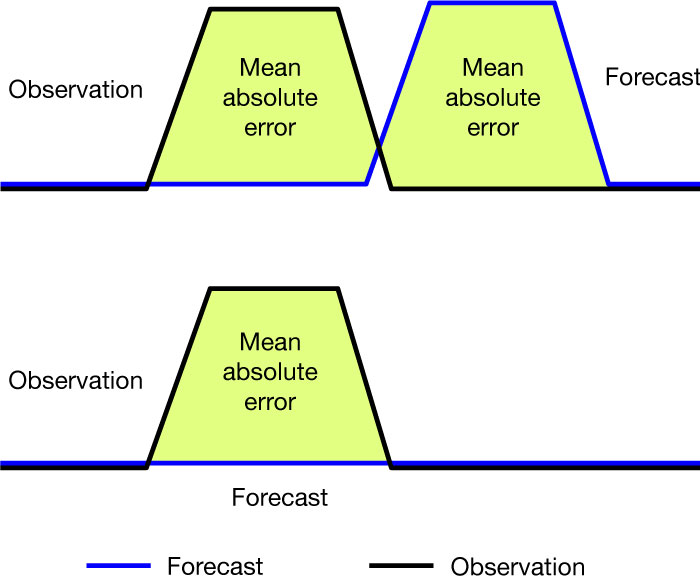
Traditional verification metrics, such as the mean absolute error (MAE) or the root mean square error (RMSE), compare forecasts and observations individually at each location. That becomes a problem when an event such as a heavy rainfall is forecast slightly off the location where it actually occurred. A forecast predicting a feature with sharp gradients will be doubly penalised if it predicts the feature at a wrong space or time: once for missing the feature in the correct spot, and once for the false alarm in the wrong place (Figure 1).

Figure 1 Illustration of the double penalty effect: a forecast that is able to predict an observed feature but not its exact location (top panel) has a higher mean absolute error than a forecast with no feature (bottom panel).

Hence the error will be twice as large as for a forecast that does not predict the feature at all. You would agree that there is more value in the wrong-location forecast than in the flat one, especially if the displacement error is small. Indeed, if you were to issue warnings or assist decision making, you would definitely have a look at neighbouring point forecasts, rather than interpreting the grid-point values literally.

One way of dealing with the double penalty issue is to compute scores that rely on neighbourhood analyses of different sizes instead of just point-wise. In the last decade, the limited-area modelling community has developed many spatial verification techniques. We are testing one of these, the Fractions Skill Score (FSS), as part of the move of ECMWF towards global km-scale modelling under the EU’s Destination Earth initiative. It gives a more complete picture of forecast performance for fields such as precipitation or cloudiness, which may exhibit little skill at the grid scale but significant skill at larger scales. It also provides a natural framework for comparing forecasts at different resolutions, which is needed for km-scale model development and evaluation.

The Fractions Skill Score

The FSS is a spatial verification technique that does not automatically penalise location errors such as the one depicted in Figure 1. It answers the question: did the observed feature occur in a nearby location in the forecast?

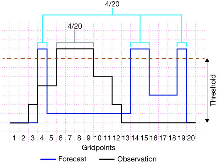
To do so, we count the fraction of grid points in a neighbourhood at which a given threshold (e.g. of precipitation amount) is exceeded, both in forecasts and in observations (Figure 2). Then we compare the two fractions by computing their squared difference. The neighbourhood analysis is done separately at each grid point and then averaged over the region of interest.

The FSS is then obtained by normalising by the worst score that could be obtained from rearranging the forecast fractions field. The FSS must be computed for multiple thresholds and neighbourhood scales to get an idea of the spatial scales at which the statistics of the number of exceedances in the forecasts match the statistics of the observations. By constraining the statistics to a neighbourhood, the FSS requires some degree of association at larger scales, while allowing for smaller-scale location and shape errors.

Figure 2 The Fractions Skill Score measures the squared difference of the number of exceedances above a certain threshold over a neighbourhood. In this simplified one-dimensional example, the model and observations agree perfectly in this neighbourhood of 20 grid points.

How to interpret the FSS results

Despite its name, the FSS is not a traditional skill score that measures improvement over a fixed reference forecast. It ranges between 0 and 1, and positive values do not automatically mean that the forecast is useful. In most cases, a threshold of FSS = 0.5 may be a useful lower limit, although FSS values below 0.5 may still be regarded as useful for some applications if the forecasts are not perfectly calibrated.

If the number of threshold exceedances in the forecast and observations are overall different due to imperfect calibration of a forecast, this will be penalised. In such cases, it is desirable to use quantile thresholds instead of absolute thresholds.

Verification of HRES precipitation

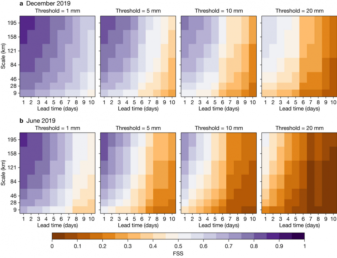
We have assessed the skill of daily-accumulated precipitation forecasts from the ECMWF operational high-resolution global forecast (HRES) over Europe for different thresholds in a summer and a winter month of 2019 (Figure 3). The observational dataset used for this evaluation is GPM-IMERG, a satellite-based, gauge-corrected gridded precipitation product providing data every 30 minutes with a spatial resolution of 0.1 degrees.

Each panel in Figure 3 shows the FSS as a function of forecast lead time and neighbourhood scale from the grid-scale up to about 200 km. As expected, skill increases with scale at all lead times. Values above 0.5 (in purple) indicate that the forecast is useful at that scale. At a threshold of 1 mm in winter (leftmost panel of Figure 3a), the HRES is skilful for nearly all lead times and scales shown. In summer (leftmost panel of Figure 3b), forecast skill is lost after about 8 to 9 days, even at larger scales of 100 to 200 km.

Moving to higher thresholds, the FSS generally decreases, so that at 20 mm some skill is left only in the short range and at large scales in winter, and little skill in summer. Generally, there is a substantial gain in skill when moving from the grid-scale to the next-bigger scale (boxes with 3x3 grid points).

Figure 3 Fractions Skill Score of HRES precipitation forecasts over Europe for four thresholds, presented at multiple spatial scales and for lead times of up to 10 days ahead, for (a) December 2019 and (b) June 2019. Purple colours indicate a useful spatial scale at particular lead times.