
Machine learning is playing an increasing role in weather forecasting: forecast trajectories can be based on it entirely, or machine learning can be used to improve the initial conditions and the trajectory of physics-based forecasts.
Here, we present some of the progress that has been made on the second front. These developments are part of a bigger drive at ECMWF to combine physics-based models with observation-driven machine learning models.
The aim is to go beyond current forecasting skill barriers while retaining the realism and interpretability of our forecasts. The changes will be incorporated in the ECMWF operational forecasting system starting next year.
These efforts are in addition to ECMWF’s development of purely machine-learning-based forecasting techniques, which recently have seen the introduction of ensembles. They are also separate from attempts to produce weather forecasts directly from observations using machine learning.
Correcting model error in the initial conditions
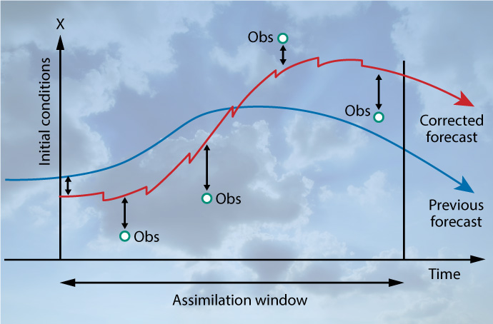
We use a technique called 4D-Var that assimilates observational data into our weather model to establish the initial conditions of forecasts. 4D-Var adjusts a short-term forecast slightly so that it better fits the weather observations made over a recent period of time, called the assimilation window.
The short-term forecast is called the ‘first guess’ or ‘background’, and the updated new trajectory the ‘analysis’.
In traditional ‘strong-constraint’ 4D-Var, it is assumed that the model is perfect. In ‘weak-constraint’ 4D-Var it is recognised that it is not, and some adjustments are made.
“At some point you realise that there are systematic differences between the model and certain observations, and you have to account for the fact that the model may be consistently wrong in specific weather situations,” says ECMWF scientist Massimo Bonavita.
Traditionally, the adjustments are by a fixed amount per time increment, as shown in the diagram below:

In data assimilation, a previous forecast, here called ‘first-guess trajectory’, is replaced by a corrected forecast, called the ‘analysis trajectory’. Traditional weak-constraint 4D-Var applies constant changes η to the analysis trajectory to remove bias from it as far as possible.
However, machine learning tools can be used to vary the adjustments to account for model errors. Also, while corrections only used to be applied in the stratosphere, now they are going to be applied in the troposphere as well.
“This is a more difficult problem because the model errors are smaller, but they are still significant, especially in the boundary layer of the atmosphere and close to the interface of the atmosphere with land and ocean surfaces,” Massimo explains.
The boundary layer is the part of the atmosphere that is directly influenced by the Earth's surface. “Here, it is important to have error corrections that vary throughout the day.”
The following animation illustrates the variable corrections of near-surface temperature tendencies per hour that are going to be applied in the new data assimilation system, compared to constant tendency corrections:

A time series of constant tendency correction and time-dependent tendency correction of near-surface temperature between 00 UTC on 20 July 2022 and 10 UTC on 24 July 2022. The constant tendency correction includes small changes for every 12-hour assimilation window. (Time series courtesy of Patrick Laloyaux, ECMWF)
These changes are scheduled to be implemented as part of Cycle 50r1 of the Integrated Forecasting System (IFS), to be introduced in 2025.
Correcting model error in the forecast
Work is also going on to correct model errors during the forecast. “The idea is to extend weak-constraint 4D-Var, using a neural network to correct for systematic errors of the model during the forecast rollout,” Massimo says.
The neural network doesn’t just deliver an estimate of model errors but provides a model of them, the state of which depends on the actual weather situation. This means that it can be applied to any configuration of the model.
With this use of machine learning, the main evolution of the forecast is still represented by the physics in the IFS.
“We are in effect introducing a small correction term that accounts for systematic errors of the model,” Massimo says. “The output that you get is still a fully consistent physical field.”
Tests of the impact on forecasts show a positive effect on almost all predicted variables and forecast ranges.

Tests show improvements (blue) over the current forecasting system for a wide range of variables and forecast ranges in the northern and southern extratropics, using ECMWF’s analysis as verification. Results are shown for anomaly correlation and root-mean-square (RMS) error/standard deviation of error. The outcome is more mixed in the tropics. (Image courtesy of Marcin Chrust, ECMWF)
This is still work in progress and will be implemented in a future IFS model cycle.