A new set of machine-learning-based forecasts is now available through the ECMWF web charts. The newcomer’s name is FuXi, from researchers at Fudan University and Shanghai Qi Zhi Institute in Shanghai, China. FuXi is actually a cascade of machine learning (ML) models where each “sub”-model is optimised for a specific forecast time window. Like Graphcast, Pangu-Weather, and FourCastNet, also available on the ECMWF website, FuXi is trained on ERA5 and has a spatial resolution of 0.25° (approximately 31 km). However, FuXi is based on 3 different models, each one optimised for a different time range: 0–5 days, 5–10 days, and 10–15 days.
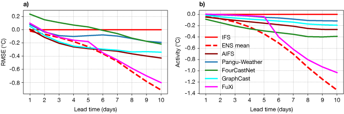
The cascade of models aims at improving scores in the medium range while maintaining performance at shorter lead times. Looking at the scores averaged over three months (June–July–August 2023), the cascade strategy seems efficient as we see better root-mean-square error (RMSE) for FuXi compared to other ML models and the Integrated Forecasting System (IFS) for forecasts of temperature at 850 hPa (T850) for the time window of 5–10 days. However, a better RMSE comes at the “cost” of a lower forecast activity due to smoothing as discussed below. In Figure 1, we plot differences with respect to the IFS statistics, where in a) the smaller the RMSE, the better the forecast, and in b) the lower the activity, the less variability in the forecast. Results for the IFS ensemble (ENS) mean are also included in the plots as they are an important part of the discussion.

Figure 1: Difference with respect to IFS statistics: a) RMSE (the lower, the better) and (b) forecast activity (the higher, the more active) for temperature at 850 hPa (T850) averaged over 1 June 2023 to 31 August 2023, northern hemisphere.
An instance of the bias/variance trade-off
The bias/variance trade-off is a well-known conundrum in the ML community. On the one hand, one should aim for the best possible fit on the training dataset (when building the model), but on the other hand, one should have a model that generalises well on the validation dataset and to future unknown data (when the model is used to make a prediction).
The RMSE/activity trade-off can be seen as a variant of the bias/variance trade-off. At the same time, one should aim for 1) a forecast that minimises the squared difference with the targeted “true” atmospheric state, as measured with a loss function (the RMSE, for example) and 2) a forecast that “resembles” the true atmosphere (in terms of variability and extremes), that is, with the right level of activity. Unfortunately, characteristics 1) and 2) cannot be captured at the same time with a single forecast at longer time ranges. This statement can be demonstrated mathematically but can also be intuitively understood.
The longer the forecast range, the more difficult it is to make an accurate forecast because of the chaotic nature of the atmosphere. The predictability of weather events is indeed generally lower at longer time ranges. When the uncertainty about the future state of the atmosphere is large, a (deterministic) forecast that makes bold predictions might be severely penalised: a penalty for predicting events at the wrong place (or with the wrong timing) and a penalty for missing the events that actually occurred. In verification, this situation is referred to as the double-penalty effect. As a consequence, smoother forecasts that are not realistic scenarios (like the ensemble mean) provide on average lower forecast errors in the case of less predictable weather situations.
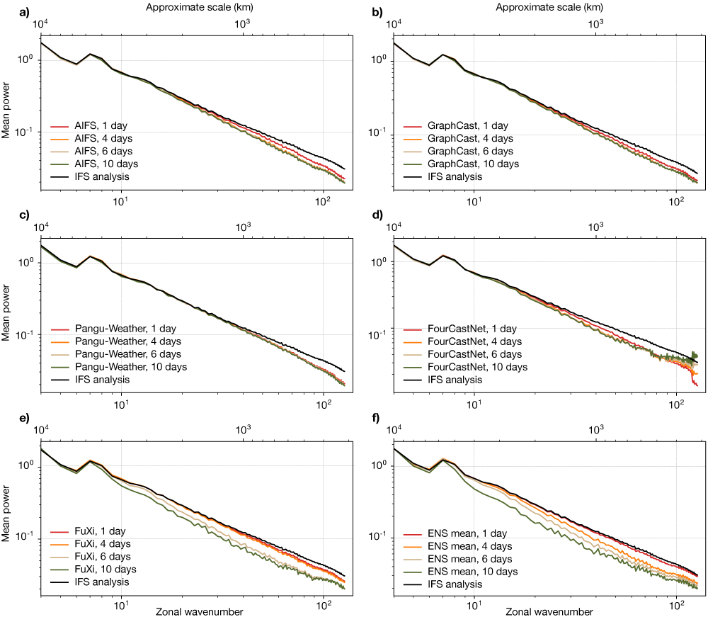
Forecast smoothness can be diagnosed with a power spectra analysis. Figure 2 shows the level of energy at different scales in forecasts at different lead times. Close to the forecast start time, the ML-based forecasts have a spectrum comparable to that of the IFS analysis. At longer lead times, we observe less energy at smaller scales (the scales that are less predictable) for all ML-based forecasts (this is not the case for the IFS forecast, which has a spectrum that barely changes with lead time, not shown here). This loss of energy at synoptic scales is particularly strong at day 6 and day 10 for FuXi and the ENS mean in Figure 2(e) and 2(f). The good performance of FuXi in terms of RMSE is directly related to its forecast characteristics in terms of smoothness.

Figure 2: Power spectra of forecasts for geopotential at 500 hPa (Z500) from different ML models and the ENS mean at day 1, 4, 6, and 10, compared with the spectrum of the IFS analysis (black line).
Ensemble forecasting as a way forward
FuXi forecasts share more similarities with the ENS mean than with any of the other deterministic forecasts. For some applications, an ensemble-mean type forecast is the best choice, but for other applications, more information (or different information) is needed. For example, forecast uncertainty is a key piece of information for decision-making. Whether a forecast has a good chance or not of materialising influences dramatically the way a forecast is eventually used in practice.
In the weather and climate community, the Monte-Carlo method is the favoured way to approach probabilistic forecasting. An example of its application is the IFS ensemble: a set of weather scenarios, each one representing a plausible and realistic state of the Earth system, which together capture the uncertainty of the forecast of the day. From an ensemble, one can derive the ensemble mean, which is the optimal forecast when aiming at a minimisation of the RMSE. Also, the double-penalty concept does not hold in an ensemble framework because a single forecast is substituted by a set of forecasts whose variety represents the forecast uncertainty (in space, time, and amplitude). Proper scores are used to assess probabilistic forecasts: they are minimised when the forecast uncertainty reflects adequately the forecast potential error. In other words, the ensemble approach solves the RMSE/activity dilemma: the ensemble mean minimises the RMSE while the ensemble members are realistically “active” scenarios.
Ensemble forecasting based on ML models is an active field of research. With FuXi, we see that targeting directly longer time ranges does not provide realistic scenarios, but instead a good estimate of an ensemble mean. A rollout using shorter time windows would allow more realistic forecasts but with fast-growing errors that should be compensated for by an accurate representation of the model and initial condition uncertainty. The contributions and representation of these sources of uncertainty in generating reliable ML-based ensembles remain to be explored.
Authors
Zied Ben Bouallegue and the rest of the AIFS team (Mihai Alexe, Matthew Chantry, Mariana Clare, Jesper Dramsch, Simon Lang, Christian Lessig, Linus Magnusson, Ana Prieto Nemesio, Florian Pinault, Baudouin Raoult, Steffen Tietsche)
