How ensemble forecasts enhance the energy sector

Isla Finney

Lake Street Consulting Ltd

Use of ensemble forecast information is now so commonplace in the energy sector, many don’t remember making decisions without it. However, my recollection of the early 2000s was a focus on the op runs. 2000-2005 saw a gradual introduction of ensemble means, with use of probability information more widespread by 2010. Over the last decade, there has been increasing use of ensemble member information, including the exploration of how regimes impact on energy supply/ demand balances.

Ensemble members lend themselves to use in the energy sector, where temporal and spatial coherence is needed to forecast supply/demand balances – in power, gas, oil and coal. The rapid expansion of renewable energy production has meant that a good weather forecast is key for good decision making in power markets. Understanding why requires a reasonable knowledge of the within day power demand profile and start-up times of various thermal plant is required, and was considered beyond the brief talk at this meeting. A simpler example was used: the cumulative gas demand – over the period of the forecast – for a hypothetical gas supplier in the UK.

Gas demand is influenced by weather in two main ways: the residential (or Local Distribution Zone) demand for heating and gas needed for power stations. At first order, the influences are the effective temperature (of the house walls) and the wind generation off-setting the need for gas turbine generation. Industrial gas demand is not considered, since it is largely weather independent. Using a simplified model for each weather dependent component, we can convert a weather forecast into a daily gas demand forecast, as shown in Figure 1.

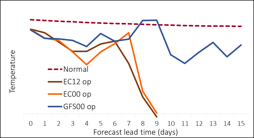
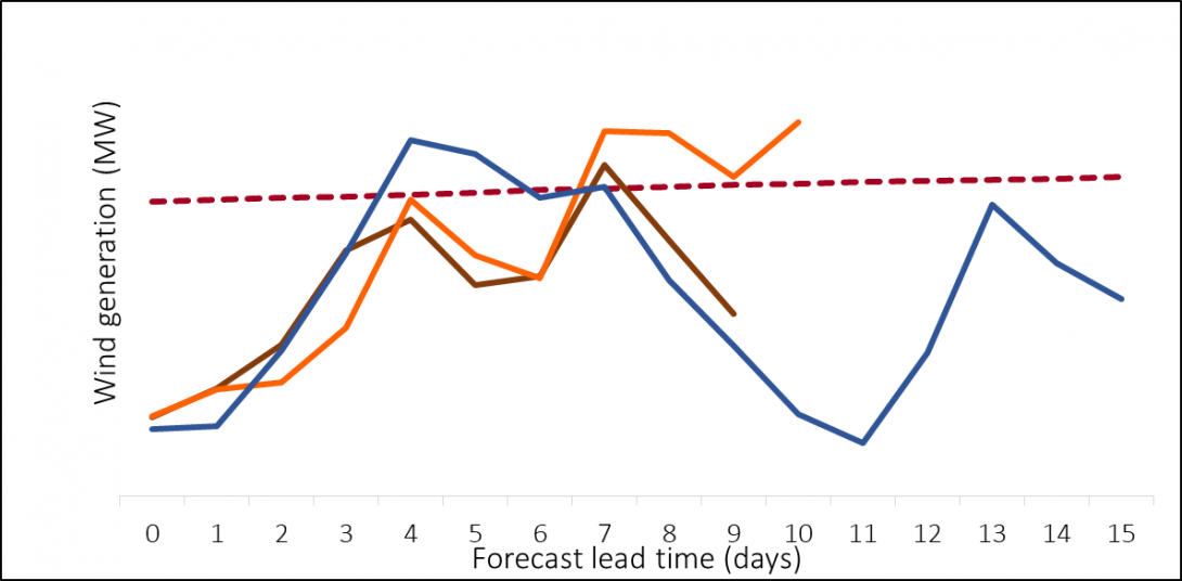
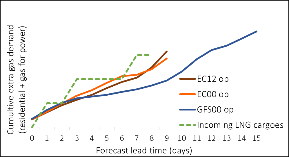
If we suppose that piped gas provides the normal gas demand and LNG cargoes are required to meet the extra (above normal) gas demand, the weather forecast can help decide when to tender for LNG cargoes. In Figure 1, the incoming LNG cargoes meets the extra demand forecast by the EC op (high resolution operational run), and exceeds the extra demand suggested by the GFS00 op forecast. From the op runs, it would therefore seem that no extra LNG cargoes are required.

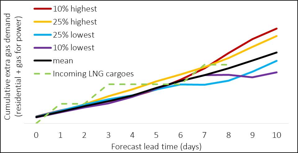
If we then have access to the EC ensembles, we can take the 10% highest gas demand at day 10, and similarly for other levels. This gives us Figure 2, which shows that for the majority of ensemble members, an additional LNG cargo would be required to meet demand. What’s important here is that we keep the information of how each ensemble member evolves, not only its value at the end time.

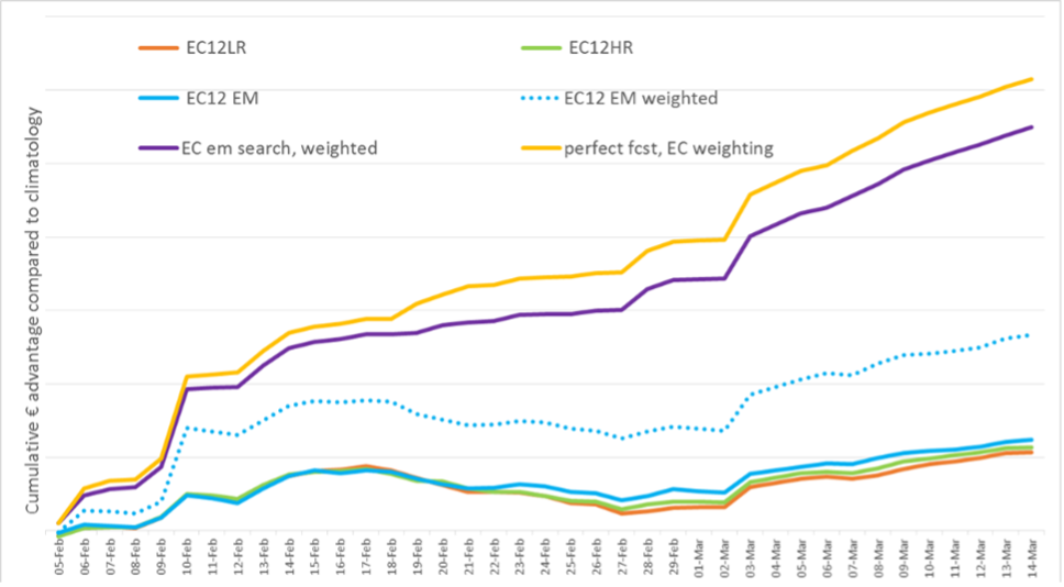
The above is an example of a single forecast initialisation time. Whilst that example hasn’t been generalised, an example of looking at the value of ensembles in wind forecasts for Italy at a 4 day lead time was a first step towards trying to capture the value of the ensembles over a month of forecasts and is shown below in Figure 3. By weighting the ensemble mean by the inverse of the ensemble spread, the value of the ensemble information increases significantly.

Whilst it is my understanding that much research happens in-house within the sector, little is published in peer-reviewed journals about the value of ensembles in the energy sector. Two students at AOPP have written papers with Tim Palmer, Antje Weisheimer and I: Stanger et al., (2019) and Dorrington et al., (2020).