In the last few years, ECMWF’s post-processing capabilities have been substantially extended. Part of this success has been the development of the internal interpolation package MIR (Maciel et al., 2017). This is the post-processing engine behind both product generation (pgen) and the client to access the meteorological archive (MARS). Metview, ECMWF’s software for accessing, manipulating and visualising meteorological data, has for many years given access to the same post-processing features.
MIR provides sensible defaults, such as interpolation methods and their parametrization, for the roughly 5,000 parameters in the GRIB parameter database (https://apps.ecmwf.int/codes/grib/param-db). More recently, developments in Metview have leveraged MIR’s more sophisticated regridding functionality. In this article, we shall explore how these features allow users to post-process their parameters of interest beyond the default behaviour for improved results.
Why regrid data?
Why would users want to regrid data? There are many reasons, and users will have their own. The most common is the need to have data from multiple sources, such as datasets and different models or versions of them, in the same geographical representation. Other reasons include reducing the data volume that needs to be transferred or stored, or the need to manipulate the data with specific workflows, for example machine learning. Some workflows will require the data to be stored in a simple regular lat/lon grid, so the output from most numerical weather prediction (NWP) models would need to be regridded in order to be used.
Metview’s Regrid module
Metview is an open-source user-facing application developed at ECMWF for exploring and post-processing data related to meteorology. The graphical user interface (GUI) provides a wide range of functionality tailored towards exploring data and developing workflows. Metview’s Python interface is open to integration with other applications and communities in many areas, and it can be used in batch, interactive and Jupyter environments. Metview already used the same postprocessing engine as the one used in MARS and pgen in its ‘Grib Filter’ module, but recently the engine was more tightly integrated with Metview for advanced functionality via the new Regrid module. This article focuses on this additional regridding functionality.
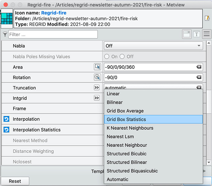
Regrid provides Metview with new functionality both in Python and Macro. When run from the GUI, it also has an interactive editor with dynamic properties, designed to encourage exploration. Only a selected few options are initially available, but with a few clicks these options expand, allowing precise specification of how you want your data to be processed (Figure 1).
%3Cstrong%3EFIGURE%201%3C/strong%3E%20The%20Regrid%20icon%20editor%20in%20the%20GUI%20has%20many%20dynamic%20options.FIGURE 1 The Regrid icon editor in the GUI has many dynamic options.
Interpolation is a very broad topic, and many options that are relatively sophisticated will require further explanation. There are newly introduced methods: a long-awaited conservative method, a series of statistical methods, and finally, advanced k-nearest neighbours interpolation methods. The handling of special values embedded in parameters provided by ECMWF, representing masks and missing values, is also significantly improved and is user controllable. In addition, there is introductory geographic information system (GIS) support.
Choosing an interpolation method
Data has a meaning and is produced with an intent. It is up to the user to know how to use the data, how to explore it and which information is important. It really depends on the application; the solutions are not the same for everyone. In addition, regridding or postprocessing in general are destructive procedures.
The objective is to preserve most of the signal when processing data. If the field values represent an alert level, then the maximum value in each grid box should likely be preserved. For categorical data, such as vegetation type, consider whether the most common value in a grid box is the one to be preserved. With increasingly large datasets, it helps to be familiar with post-processing techniques in order to extract the most value.
Statistical interpolation
Statistical interpolation is not interpolation in the classical sense, in that the resulting value does not come from a geometrical interpretation of field values, but rather as the statistic of interest from contributing (neighbouring) points.
There are many parameters for which the statistics of interest are maximum, minimum, or mean, such as when handling temperature, alert level, wind gust, precipitation, etc. Other statistics available are count (unlimited or above/below a threshold), standard deviation, variance, skewness, kurtosis, median and mode. Figure 2 shows how the grid-box maximum method preserves high fire danger index values.
Two possible (and available) ways to choose contributing values are the grid-box and Voronoi methods. The grid-box methods simply capture all the source points that lie within a given target grid box. While this is fairly classical and well documented (such as in https://confluence.ecmwf.int/display/CKB/Model+grid+box+and+time+step), the Voronoi diagram interpretation is a tessellation defined by a collection of source grid points closest to a target grid point, and thus each polygon of source points does not necessarily cover a regularly shaped area.
%3Cstrong%3EFIGURE%202%3C/strong%3E%20Fire%20danger%20index%20data%20for%20Crete%20in%20the%20Mediterranean%20(a)%20on%20its%20original%20grid,%20(b)%20interpolated%20with%20the%20nearest%20neighbour%20technique,%20and%20(c)%20interpolated%20with%20the%20grid%20box%20maximum%20technique%20to%20preserve%20the%20highest%20warning%20levels.%20In%20all%20plots,%20the%20central%20points%20of%20the%20target%20grid%20boxes%20are%20marked%20in%20green.FIGURE 2 Fire danger index data for Crete in the Mediterranean (a) on its original grid, (b) interpolated with the nearest neighbour technique, and (c) interpolated with the grid box maximum technique to preserve the highest warning levels. In all plots, the central points of the target grid boxes are marked in green.
Conservative interpolation
The grid box methods interpret a region in space as represented by central points and an associated range in longitude and latitude, up to neighbouring grid boxes. A single grid box is therefore a rectangular region in latitude/longitude centred on a grid point. This is a tessellation comprised of regions of interest around each point, so one can perform statistical interpolation (the grid box statistical interpolation method) similar to the Voronoi statistics method previously described. The grid box interpretation, however, is not extendable to arbitrary sets of points, so it is only currently available for structured, unrotated grids.
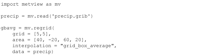
Grid boxes are particularly useful for calculating integrals and fluxes when assuming constant values per grid box. This is the basis for grid box conservative interpolation: for one target grid box, which defines its contributions from the area of intersection of the source grid boxes, one preserves the integral of the source grid boxes to the target grid box (Figures 3 and 4). This method is not only globally conservative but also locally conservative. It is only up to first-order accurate, but even so it is suitable for many parameters of interest, such as fluxes (ECMWF’s Integrated Forecasting System produces many) or integral parameters (such as total column parameters), including precipitation-related parameters, tracers, and aerosols among others. The Copernicus Atmosphere Monitoring Service (CAMS) operated by ECMWF provides a comprehensive list of these types of parameters (https://atmosphere.copernicus.eu).
%3Cstrong%3EFIGURE%203%3C/strong%3E%20Precipitation%20over%20six%20hours%20in%20southern%20Britain%20and%20northern%20France%20(a)%20on%20its%20original%201%C2%B0/1%C2%B0%20grid,%20and%20(b)%20interpolated%20to%20a%205%C2%B0/5%C2%B0%20grid%20using%20the%20grid%20box%20average%20technique.%20The%20value%20of%20each%20resulting%20grid%20box,%20such%20as%20the%20one%20highlighted%20in%20red,%20is%20the%20spatially-weighted%20average%20of%20the%20source%20grid%20boxes%20that%20cover%20its%20area,%20meaning%20that%20total%20quantities%20are%20conserved%20within%20each%20grid%20box%20and%20over%20the%20entire%20data.FIGURE 3 Precipitation over six hours in southern Britain and northern France (a) on its original 1°/1° grid, and (b) interpolated to a 5°/5° grid using the grid box average technique. The value of each resulting grid box, such as the one highlighted in red, is the spatially-weighted average of the source grid boxes that cover its area, meaning that total quantities are conserved within each grid box and over the entire data.
%3Cstrong%3EFIGURE%204%3C/strong%3E%20Python%20code%20to%20regrid%20precipitation%20GRIB%20data%20using%20the%20conservative%20grid%20box%20average%20method%20to%20produce%20data%20on%20a%205%C2%B0/5%C2%B0%20grid%20on%20a%20subarea.FIGURE 4 Python code to regrid precipitation GRIB data using the conservative grid box average method to produce data on a 5°/5° grid on a subarea.
Advanced k-nearest neighbours interpolation
In some cases, the representation of points in space is better interpreted without structure (a disjoint cloud of points). In that case, the source values contributing to a target point depend on how far away they are. The k-nearest neighbours interpolation controls two aspects: how the source points are selected (relative to a target point) by distance or number, and how these selected points are weighted (calculation of their contribution).
Distinct ways of selecting the source points are:
by number (k), irrespective of distance
by distance/radius, irrespective of number
by number and up to a distance (intersection of sets by number and distance)
by number or up to a distance (union of sets), and
by sampling points selected by distance.
To control how the selected points contribute, one common method is inverse distance weighting (IDW) with contributions calculated as a weighted average based on distance (more distance assigns less weight). The Shepard method is the general case of this: it defines IDW, IDW squared, and IDW to a user-specified power. Another type is distance-free weighting, which is just straightforward averaging. It does not employ distance and therefore is relevant where different resolutions are used for the same workflow, suitable for machine learning applications training at lower resolution and application at higher resolution. And finally, special options exist distributing weighting according to distance over a Gaussian curve (user-defined by standard deviation, centred on each target point), or for specific purposes such as handling topographic data at model resolution – a smoothing operator. The following options are available:
inverse distance weighting (including the Shepard method)
distance weighting following Gaussian function curve
Several parameters might not be completely defined over the whole globe or are only defined over some specific areas. This is the case for many surface parameters, which have values only defined over land or sea. Values over other areas are routinely referred to as missing, and the handling of missing values is generally transparent to the user: they are not included when interpolating.
Points representing missing values are never involved in interpolation, and the remaining contributions are always linearly re-weighted (to sum to one). Regrid allows finer control over this handling: an output value can be set to missing if all, any or the heaviest-weighted (according to the interpolation method) of its contributing points are missing.
The control over this behaviour has a strong effect, for example, on the way land-defined values are represented over the sea on interpolation, or vice-versa. This specifically affects values near coastlines. The missing-if-any-is-missing favours missing values, missing-if-all-are-missing favours non-missing values, and missing-if-heaviest-is-missing is in between (the default behaviour). The default behaviour works better than the others across large resolution changes.
Some parameters include values that have a semantic rather than physical meaning. These include the missing values mentioned above, but also other specific values, depending how the data is intended to be interpreted. For example, sea-surface temperature (°C) has a value of 0 over land, for some products representing the absence of data, or snow depth (m) has a value of 10, representing a glacier.
These values should not interfere with the interpolation of physically relevant values. Regrid offers a mechanism to control these, by specifying a value and tolerance to compare with. This user-defined tolerance addresses a practical concern, as field values might be encoded approximately, not exactly, to the original value, especially when archived (in MARS) or stored on disk in GRIB or netCDF formats.
GIS applications
For applications where a precise description of location is required, for example because of information exchange with other data sources or producers, Regrid has support for PROJ-based projections. This wellknown library handles all kinds of cartographic projections and supports several spatial analysis applications. It is ideal for handling data from local area models with very specific projections.
PROJ support at ECMWF starts with the ecCodes ability to generate a PROJ string to describe a coordinate reference system (CRS) from GRIB-encoded data. MARS hosts a great variety of data, including many LAM model grids on a variety of projections, e.g. Lambert conformal conic (LCC), Lambert azimuthal equal-area (LAEA) and Mercator.
Regrid supports this kind of GRIB format GIS-compliant data as input, and in addition it supports built-in mappings from either PROJ strings or EPSG codes (a short, concise way to specify a CRS) to GRIB output. The assignment of CRS to specific grids needs to be agreed with data producers in advance.
As an application example, the European Flood Awareness System (EFAS) operates on a European scale to provide coherent medium-range flood forecasts, implemented by ECMWF. The EFAS workflow is supported with an LAEA grid specified with a particular EPSG code, and its products are integrated in a variety of GIS workflows. With this added support, Regrid results are well integrated either as a source to, or target from, EFAS products.
Using templates
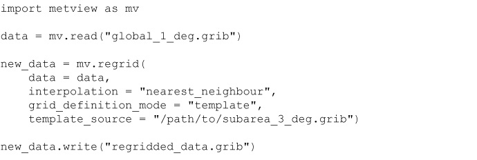
A common task is to put GRIB file ‘A’ onto the same grid as GRIB file ‘B’. Regrid can simplify this process by allowing the use of a template GRIB. Instead of supplying the various parameters required to reproduce the target grid, the user can provide a sample GRIB file, and its grid parameters will be read and used to generate the output (Figure 5).
%3Cstrong%3EFIGURE%205%3C/strong%3E%20Python%20code%20to%20regrid%20one%20GRIB%20file%20using%20another%20as%20a%20template.FIGURE 5 Python code to regrid one GRIB file using another as a template.
Availability
Metview is installed on ECMWF’s computing platforms including the Member and Co-operating State server ECGATE. For use external to ECMWF’s computing platforms, Metview is also available as a binary installation on the conda platform, available through the conda-forge channel with one of these commands:
conda install metview -c conda-forge
conda install metview-batch -c conda-forge
# no GUI installed
The Python interface can be installed with either of these commands:
conda install metview-python -c conda-forge
pip install metview
Metview’s Python documentation has been moved to readthedocs and can be accessed here: https://metview.readthedocs.io/en/latest/. A Jupyter notebook containing the examples described in this article can also be found there.
Further reading
Maciel, P., T. Quintino, U. Modigliani, P. Dando, B. Raoult, W. Deconninck et al., 2017: The new ECMWF interpolation package MIR, ECMWF NewsletterNo. 152, 36–39.